Automap4 Operator Guide

This guide explains the automap4 main window, menus, and the standard workflow for S-curve discovery, PRBS identification, closed-loop supervisory control, recording, and reporting. The screenshots use the light theme because it prints and embeds better in documentation.

Top Toolbar / Status Bar

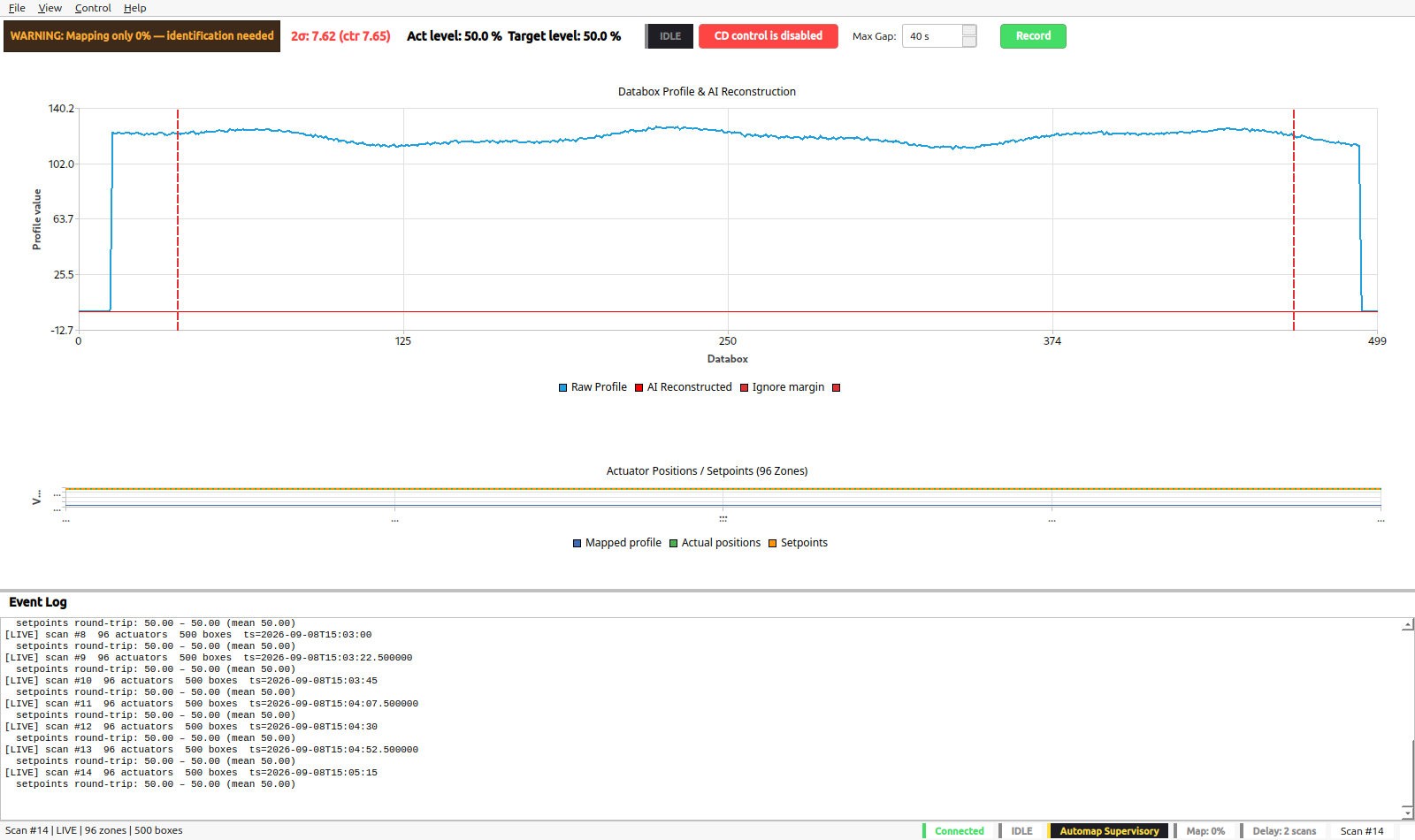
Figure 1: automap4 main window (light theme).

Primary control buttons

• Start PRBS / Stop PRBS (Ctrl+Space) — Opens the PRBS Identification dialog. PRBS teaches automap4 the mapping between each actuator and the profile response. It cannot start until a measured S-curve exists (Discovery → PRBS → Control).
• CD control is disabled / CD control is allowed / Supervisory ON — Toggles closed-loop CD control. Enabled once mapping progress passes the Control threshold set in the PRBS Identification dialog (default 90%).
• Record / Stop — Starts or stops recording scan data to a CSV file plus a companion .npz archive. The default filename depends on the current mode: tuning_log.csv during PRBS, control_log.csv during control, running_log.csv otherwise.

Status readouts

• Connected / Disconnected — ZMQ connection state to machinedriver.py or modelstdcom.py.
• IDLE / PRBS ACTIVE / CONTROL — Current operating mode.
• 2σ: full (centre) — Total and centre 2-sigma profile spread.
• Act level / Target level — Counted-zone actuator level and its target (see Actuator Level below).
• Map: xx% — Effective mapping progress across all actuator zones.
• Delay: x scans — Estimated or overridden transport delay in scans.
• Wander: x db — Current sheet-wander estimate.

Menu Reference

File

• Save Grade (Ctrl+Shift+S) — Overwrites the currently loaded grade .npz with the latest mapping, S-curve, and controller tuning.
• Save Grade As... — Saves a new grade .npz file.
• Load Grade... — Loads a previously saved grade or mapping file.
• Preferences... (Ctrl+,) — Opens the settings dialog.
• Exit — Closes automap4.

Grades

The Grades menu lists all grade_*.npz files found in the configured grade directory. Selecting one loads it immediately. A grade carries the measured S-curve, the mapping matrix, the controller tuning (Q/R/S/T, aggressiveness, integral, max delta_u), and the actuator-level settings. The grade is the tuning carrier.

Control

• S-Curve Discovery... — Measures the actuator-to-sheet geometry with deliberate bumps. Required before PRBS.
• Toggle PRBS (Ctrl+Space) — Opens the PRBS Identification dialog.
• Toggle Control (Ctrl+C) — Enables or disables closed-loop supervisory control.
• Toggle Recording (Ctrl+R) — Starts or stops CSV/NPZ logging.

View

• Profile Chart / Actuator Chart — Show or hide the corresponding chart panels.
• Manual Bump — Show/hide the manual bump bar for selecting zones and applying setpoint overrides.
• Log Panel — Show/hide the Event Log panel.
• Theme — Switch between Dark, Light, and Solar colour themes.
• S-Curve Mapping / PRBS Mapping / Mapped Actuator Profile / Mapping Heatmap / Wander Trend / 2-Sigma Trend — Open monitor windows.
• CSV Report... / Generate Field Report (PDF)... — Load a recorded CSV and create a printable or PDF report.
• Mapping Info... (Ctrl+I) — Shows mapping quality, controller tuning, and transport-delay estimates.

Help

• Tuning Procedure (F5) — Complete operator runbook from machine setup through steady control.
• Playback Help (F2) — Overview of replaying recorded logs in the office.
• ZMQ Playback Guide (F3) — Step-by-step guide for direct ZMQ playback.
• Save Machine Run Help (F4) — Operator guide for recording and sending site logs.
• Heatmap Help (F1) — How to read the mapping heatmap.
• View Todo List — Shows the project todo list.
• About automap4 — Build metadata and checkout instructions.
• About Qt — Qt framework version information.

Preferences Dialog

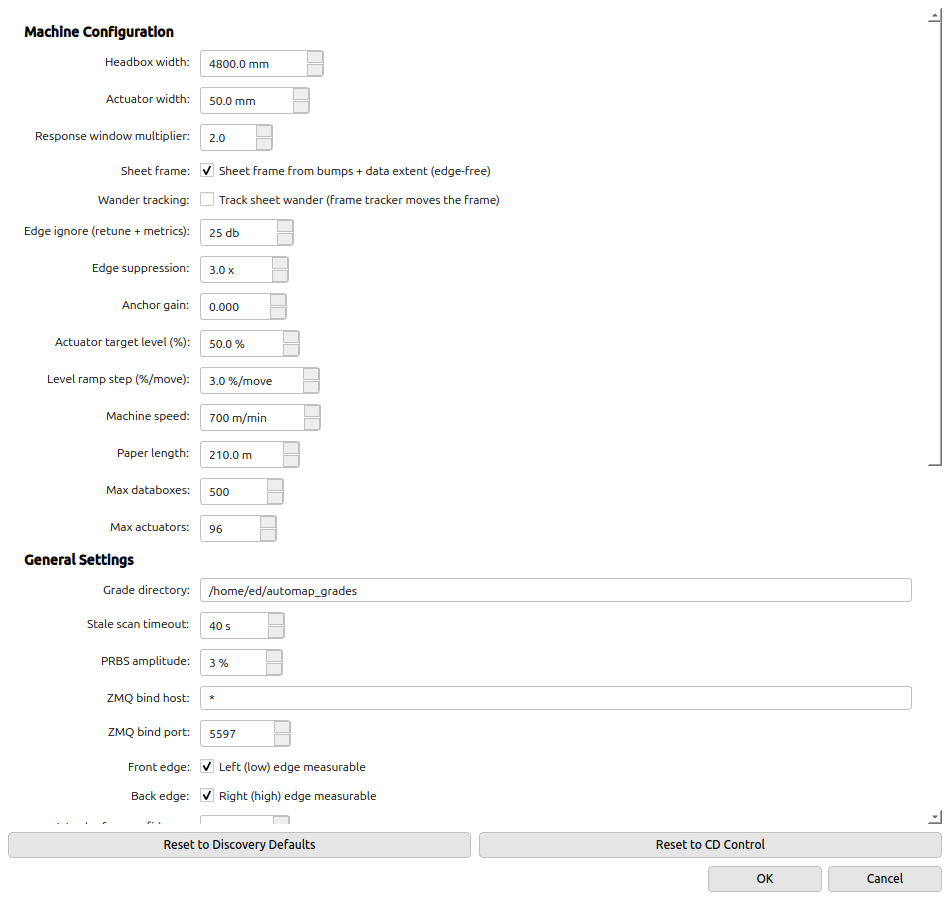
Figure 2: Preferences dialog (Machine Configuration).

Preferences are split into Machine Configuration, General Settings, and Controller Tuning. Machine identity values (headbox width, actuator width, machine speed, paper length, max databoxes, max actuators, grade directory, ZMQ bind host/port) are site identity and are not changed by the preset buttons.

Machine Configuration

• Headbox width — Physical headbox width in millimetres.
• Actuator width — Width of one dilution actuator in millimetres.
• Response window multiplier — Half-width multiplier used during PRBS correlation (default 2.0).
• Sheet frame from bumps + data extent (edge-free) — Use an actuator-anchored, edge-free coordinate frame.
• Track sheet wander (frame tracker moves the frame) — Enable the actuator-anchored frame tracker (only meaningful in edge-free mode).
• Edge ignore (retune + metrics) — Databoxes ignored at each edge for mapping retune, edge suppression, and the centre-2σ metric. Does NOT stop control.
• Edge suppression — Move-cost multiplier for edge-band actuators (default 3.0x).
• Anchor gain — Weak pull toward control-enable setpoints to prevent hours-scale drift.
• Actuator target level (%) — Target counted-zone mean level; the level is walked toward this at the ramp step.
• Level ramp step (%/move) — Maximum change of the counted-zone mean per control move.
• Machine speed — Nominal machine speed in m/min, used for transport-delay display.
• Paper length — Paper path length from headbox to scanner in metres.
• Max databoxes / Max actuators — Maximum array sizes to accept.

General Settings

• Stale scan timeout — Seconds without a scan before automap4 pauses identification/control.
• PRBS amplitude — Size of the {-1,0,1} PRBS moves in percent stroke (set in the PRBS dialog).
• ZMQ bind host/port — Where automap4 listens for machinedriver/modelstdcom connections.
• Front/Back edge availability — Whether left and/or right sheet-edge data is available.
• Wander freq confidence — Confidence level required before wander feed-forward activates.
• Throttle control by +1 scan delay — Adds one scan to the control interval for stability.
• Auto-tune controller when enabling control — Derives R/S/T from the learned mapping matrix.
• Use simple-zone control — Controls the 96-zone mapped BWT profile instead of the full databox profile.
• Dilution actuators (no bending limit) — Independent valves; no max-adjacent-difference constraint.
• Refine mapping from control moves — Closed-loop identification that updates the model during control.
• Write control debug log — Writes per-scan/per-move debug lines to control_debug.log.

Controller Tuning

• Q / R / S / T — Objective weights for target tracking, move suppression, smoothing, and absolute-profile curvature. Auto-tune derives R/S/T around Q.
• Aggressiveness (alpha) — The single tuning knob: fraction of error removed per move (default 0.70 for discovery, often 0.60 for control).
• Max delta_u — Hard per-scan actuator move limit.
• Integral gain / decay / max — Slow integral correction for persistent profile error. Use 0 gain with noisy edge detectors.

Preset Buttons

• Reset to Discovery Defaults — Loads the full discovery/PRBS recipe: edge-free frame ON, tracker OFF, PRBS amplitude 3 %, threshold 90 %, both edges available, wander confidence 100 %, edge ignore 25 db, edge suppression 3.0x, actuator target level 50 %, ramp step 3 %/move, transport delay auto, throttling OFF, auto-tune OFF, simple-zone ON, dilution ON, closed-loop ID ON, debug log OFF, Q=1.0, R=S=T=0.0673, alpha=0.70, max delta_u=9.53, integral gain=0, decay=0.98, max=0.5. A confirmation dialog warns before applying.
• Reset to CD Control — Switches to ready-to-run control mode: auto-tune ON, simple-zone ON, closed-loop ID ON, edge ignore 25 db, edge suppression 3.0x, throttling OFF, threshold 90 %, wander confidence 100 %. Grade tuning (Q/R/S, alpha, integral, max delta_u) is left untouched.

S-Curve Discovery

The S-curve is the actuator-to-sheet alignment: which databox each actuator's response lands on. It is measured, never assumed. automap4 ships no default S-curve; PRBS is blocked until a measured curve exists.

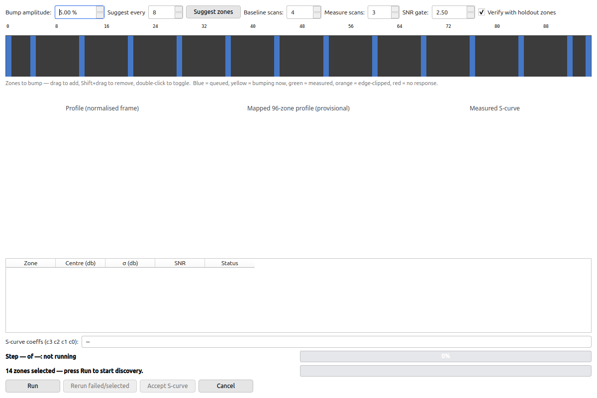
Figure 3: S-Curve Discovery dialog.

1. Open Control → S-Curve Discovery...
2. The dialog suggests a bump set. Edit it by dragging, Shift+dragging, or double-clicking zones in the bar.
3. On a noisy scanner use 7–8 % amplitude; on a clean scanner 5 % is usually enough. Press Run.
4. If no transport-delay override is set, the session first measures the delay with a mid-sheet probe bump. Answer the skip-tau question if it appears.
5. Watch the run: blue = queued, yellow = bumping, green = measured, orange = edge-clipped, red = no response. The lower chart shows the provisional 96-zone mapped profile.
6. When the fit is verified, press Accept S-curve. This seeds the mapper, unlocks PRBS, and offers to save a seed grade.

PRBS Identification

PRBS refines the discovered S-curve and learns the true response shapes. Run 30–40 scans with a verified discovery seed; you do not need the full 511-scan sequence.

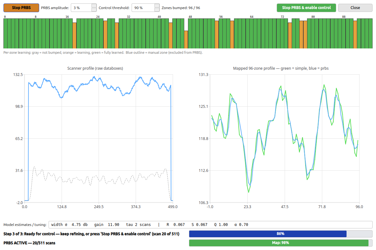
Figure 4: PRBS Identification dialog after the control gate opens.

1. Make sure Preferences carries the discovery preset (or click Reset to Discovery Defaults again).
2. Open Control → Toggle PRBS (Ctrl+Space). Set amplitude to 3 %, set the Control threshold (default 90 %), and click Start PRBS.
3. Watch the Mapping Progress bar and the per-zone quality bars: grey = not learned, orange = learning, green = fully learned.
4. When the progress bar turns green (above the Control threshold), you can click Stop PRBS or Stop PRBS & enable control.
5. Post-PRBS tuning auto-applies. Save the grade with File → Save Grade or when prompted.

Closed-Loop Control

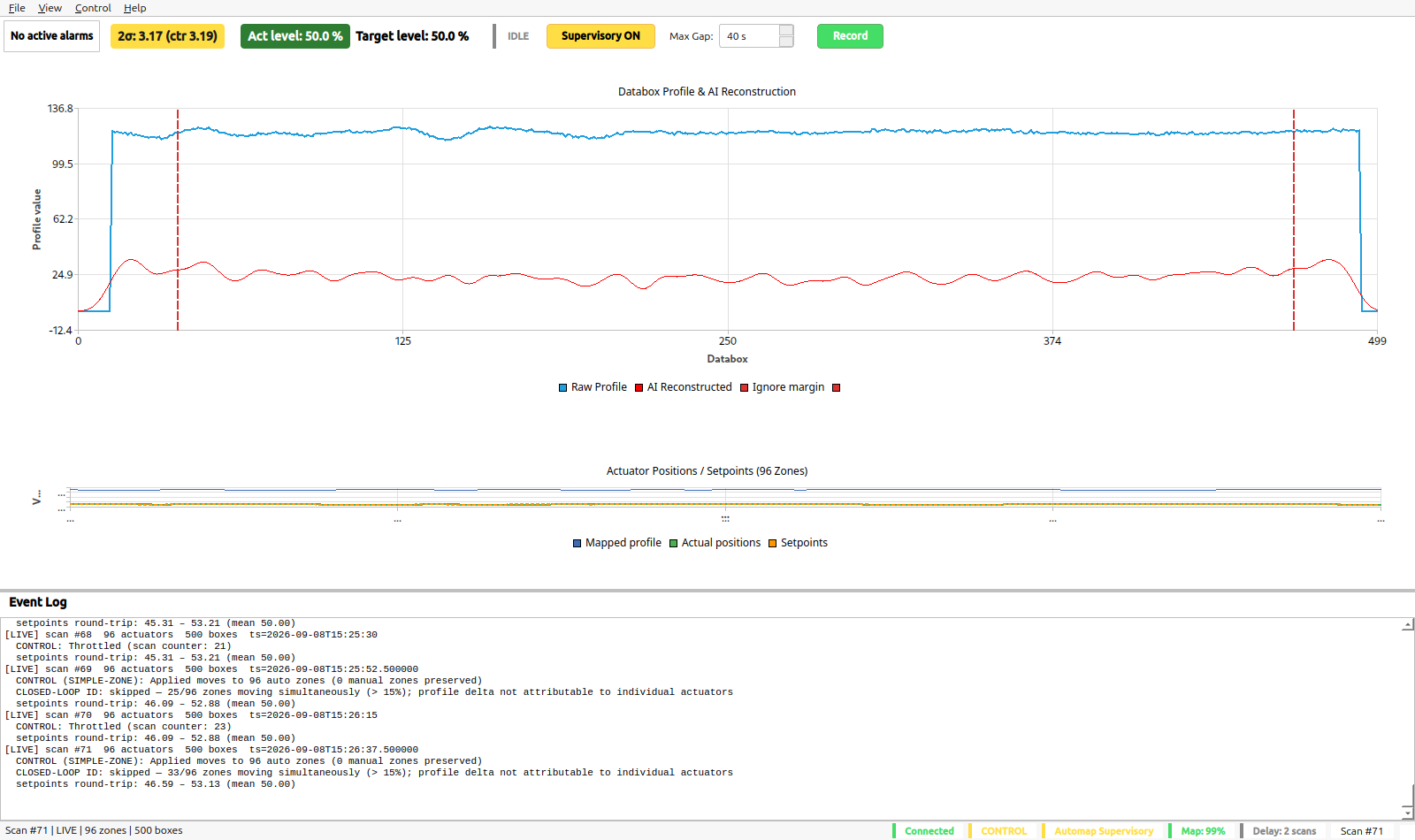
Figure 5: Main window in CONTROL mode.

1. Load the grade saved from PRBS (Grades menu or File → Load Grade).
2. Clear any manual zones. The mode badge should show CD control is allowed and Map is above the threshold.
3. Click the CD control button (or press Ctrl+C). The first time, a dialog asks whether to record; choose or accept control_log.csv.
4. The mode badge changes to CONTROL. The actuator chart shows setpoints moving as the controller flattens the profile.
5. Watch the centre 2-sigma trend. If it is too jumpy, lower alpha; if too sluggish, raise alpha. Do not change R/S/T by hand unless auto-tune is OFF.
6. To stop control, click the CD control button again or press Ctrl+C. When control stops, automap4 offers to save any mapping refinements made during control.

Mapping & Control Info

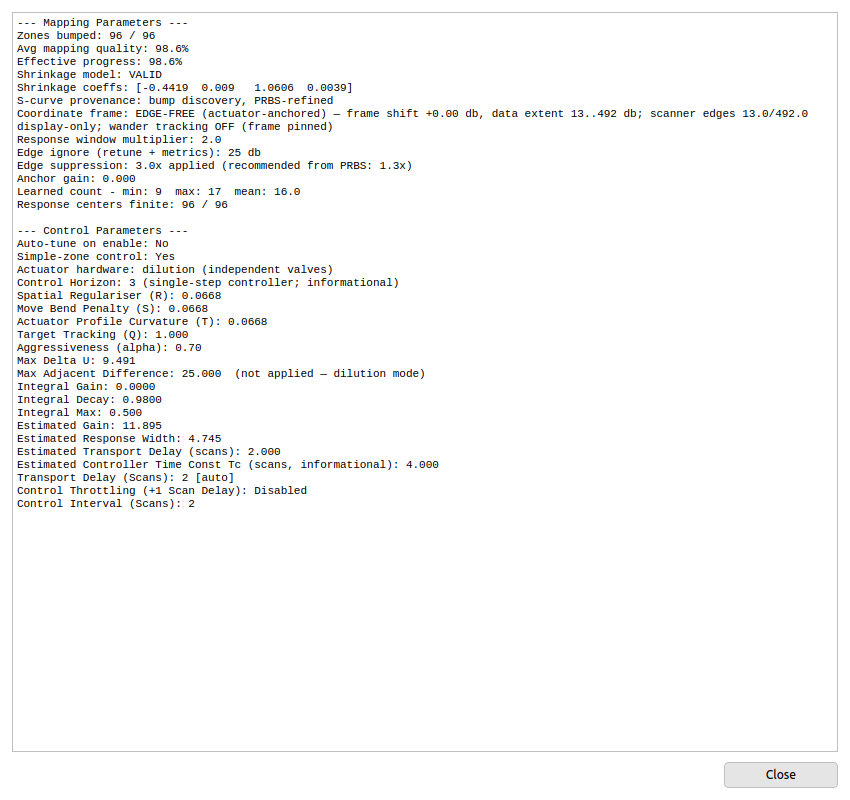
Figure 6: Mapping & Control Info dialog (Ctrl+I).

Mapping Info shows the S-curve provenance, mapping quality, learned counts, response width and gain, transport delay, and the current controller tuning. Use it after PRBS and after enabling control to sanity-check that width, tau, and the derived R/S/T are plausible.

Monitor Windows

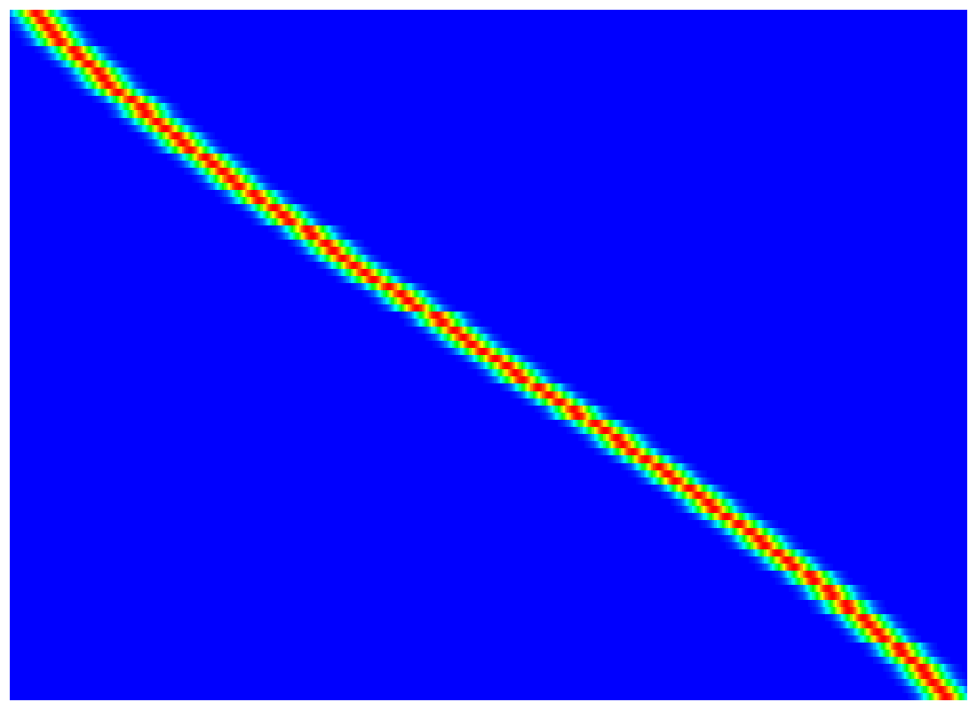
Figure 7: Mapping Heatmap.

View → Mapping Heatmap visualises the learned mapping matrix. A solid diagonal band from top-left to bottom-right means the alignment between actuators and scanner positions is correct.

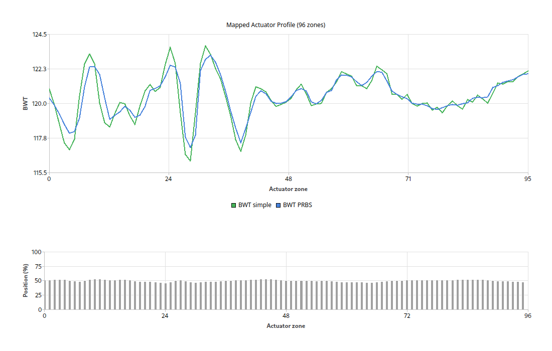
Figure 8: Mapped Actuator Profile window.

View → Mapped Actuator Profile shows the two 96-zone BWT profiles (simple zone average and PRBS-weighted) that automap4 sends back to the machine. Use it to compare the two mappings and as a cross-check for external controllers.

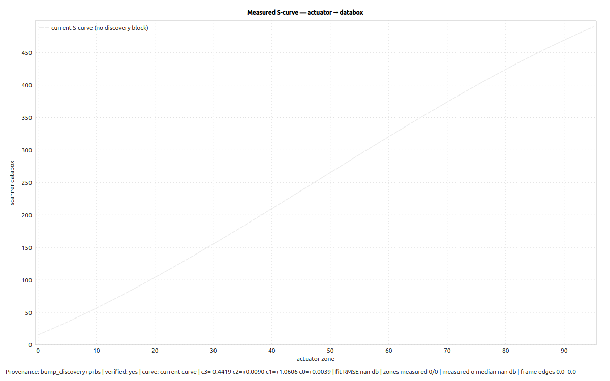
Figure 9: S-Curve Mapping window (F1 help available).

View → S-Curve Mapping shows the measured S-curve, the bumped zones ± measured sigma, and the fit readout.

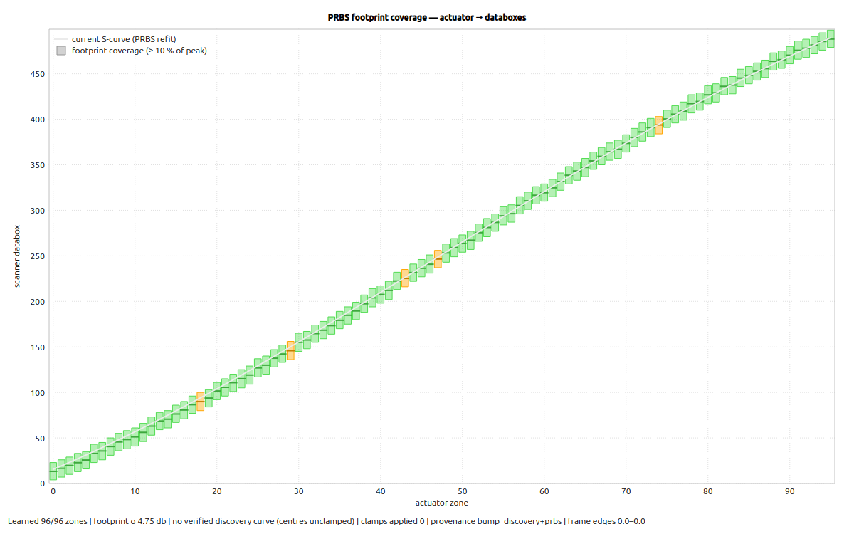
Figure 10: PRBS Mapping window (F1 help available).

View → PRBS Mapping shows each actuator's PRBS-learned footprint coverage versus the discovery curve clamp band.

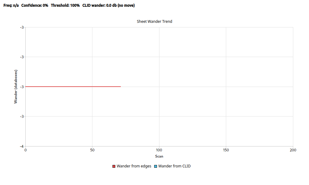
Figure 11: Wander Trend window.

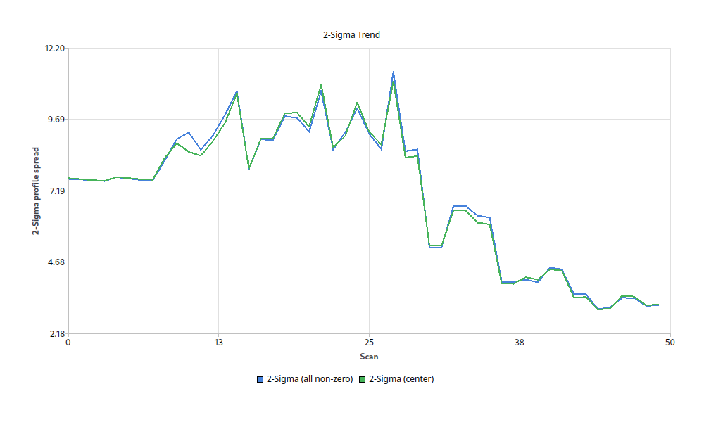
Figure 12: 2-Sigma Trend window.

View → Wander Trend and View → 2-Sigma Trend track sheet shift and profile variability over time. Use them to judge whether the controller is holding the sheet steady or whether drift is physical (wander/MD disturbance).

Recording and Field Reports

Click Record to start logging. The default filename depends on the current mode:

• PRBS active → tuning_log.csv (+ tuning_log.npz)
• Control active → control_log.csv (+ control_log.npz)
• Idle / baseline → running_log.csv (+ running_log.npz)

The CSV contains one summary row per scan. The NPZ contains the full profiles, actuator positions, setpoints, edges, machine speed, timestamps, and the learned mapping matrix.

1. Select View → Generate Field Report (PDF)...
2. Choose the recorded CSV file.
3. Choose where to save the PDF. The default name matches the CSV basename.
4. automap4 builds a PDF containing the mapping heatmap, quality distribution, 2-sigma trend, wander trend, and tuning summary.

Setting up machinedriver.py

machinedriver.py is the bridge between the real paper machine (via STEC/Multiverse) and automap4 (via ZeroMQ). In the lab, modelstdcom.py replaces the real machine's Multiverse; machinedriver.py itself does not change.

1. Launch machinedriver.py on a PC that can reach both the STEC server and automap4.
2. In the Connection group enter the ZMQ host/port where automap4 is listening (default 5555) and the STEC host/port of the Multiverse broker.
3. Open the Subscription Mapping table and map each field to the correct STEC subscription name (actuator_positions, actuator_setpoints, profile, left_edge, right_edge, machine_speed, scanner_direction). Set actuator_positions/profile/edges/speed/scanner_direction to to_zmq and actuator_setpoints to from_zmq.
4. Click Save. machinedriver will auto-connect to automap4 and start forwarding scans.
5. Use the Profile Orientation checkboxes if the scanner orientation needs reversal.

About automap4

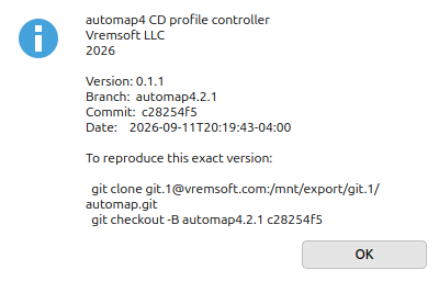
Figure 13: About automap4 dialog.

Help → About automap4 shows the package version, git branch, commit, build date, origin, and exact checkout instructions to reproduce the running version. The same build metadata is available in machinedriver and modelstdcom.